This is gonna be a fun post to write¹; it comes from a conversation a friend and I had a while back. Last year, a group of Stanford students created the Stanford Marriage Pact. Basically, people fill out a survey about themselves and then the program “[uses] a a [sic] ~nobel prize winning algorithm~ to match people with their optimal backup marriage on campus.” ² This ended up going fairly well last year, so they decided to run the Marriage Pact again this year, but this proposes a potential issue. Clearly, you’re going to marry whoever you get matched with, so what do you do if you fill out the survery both years but get matched with two different people? The only reasonable answer is that you’ll have to marry them both ³; this is simple enough until you realize that your two spouses might each have another spouse who has another spouse who … The punchline, there are about to be large groups of Stanford students all jointly married to each, but just how large of groups? More specifically, after 4 years of the Marriage Pact, will every Stanford student be apart of the same large marriage? This is (roughly) what we will investigate in this post ⁴. I will try to roughly follow the order in which I did things in my ⁵ investigations before starting this post.

Assumptions and Formalism

Let’s start by specifying the details of how we’ll model this mathematically. The first thing we’re gonna do is eliminate the need to worry about people graduating; we’ll assume the Pact matches freshman with freshman, sophomores with sophomores, and so on, and we’ll focus on a single class ⁶ instead of all students. That being said, throughout the post, assume that our class under consideration has $n=2g$ students ($n$ even) who attend college ⁷ for $m$ years (In practice, $m=4$ but 4 years may turn out to not be enough to get a connected graph with high probability). Furthermore, every student participates in the Pact each year (anecdotally, this is not too far from the truth) and everyone gets matched with someone. You are allowed to be matched with the same person each year, but matches are completely randomed, sampled from a uniform distribution.

What we have here are $m$ (undirected, simple) random graphs, $G_1,G_2,\dots,G_m$ where $|G_i|=n$ (for all $i$), each representing one year of the Pact being run (e.g. $|E(G_i)|=n$) where every vertex in $G_i$ is a student, and an edge $e=(u,v)\in E(G_i)$ means that student $u$ was matched with student $v$ by the $i$ iteration of the Marriage Pact. We want to know the probablity that their union $G=\bigcup G_i$ is connected.

First Attempt

We’ll start with an extra, very generous assumption: everyone is pansexual. So, we have some random simple graph $G=G_{n,m}$ with vertex set $V(G)=[n]:=\{1,2,3,\dots,n\}$ and the probablity that an edge $e=(u,v)$ does not exist is

\[\Pr\sqbracks{e\not\in E(G)}=\prod_{i=1}^m\Pr\sqbracks{e\not\in E(G_i)}=\parens{1-\frac1{n-1}}^m\]

since $e\not\in E(G_i)\iff u$ was matched with a student other than $v$. Let $q_{n,m}$ denote the probablity that $G_{n,m}$ is disconnected, so we’d like to be able to say something about $q_{n,m}$. Before we try and get a handle on it, we make the following useful definitions.

Convince yourself that a graph $G$ is disconnected if and only if there exists some nonempty set $S\subsetneq V(G)$ such that $E(S, \bar S)=\emptyset$. Once you have done that, consider some set $S\subseteq V(G)$ with $|S|=k$, and observe that

\[\Pr\sqbracks{E(S,\bar S)=\emptyset}=\prod_{\substack{(u,v)\\u\in S,v\not\in S}}\Pr\sqbracks{(u,v)\not\in E(G)}=\parens{1-\frac1{n-1}}^{mk(n-k)}\]

where we used the fact that there are $n(n-k)$ potential edges from $S$ to its complement. Using this, we are going to bound $q_{n,m}$ above and see what happens to this bound as $n\to\infty$.

\[q_{n,m}\le\frac12\sum_{\substack{S\subsetneq V(G)\\S\neq\emptyset}}\Pr\sqbracks{E(S,\bar S)=\emptyset}=\frac12\sum_{k=1}^{n-1}\binom nk\parens{1-\frac1{n-1}}^{mk(n-k)}\]

where the factor of $\frac12$ comes from the fact that we’re double counting pairs $\{S,\bar S\}$. Noticing that this sum is symmetric in $k$ and $(n-k)$ (and recalling that $n=2g$), we can write

\[q_{n,m}\le\sum_{k=1}^g\binom nk\parens{1-\frac1{n-1}}^{mk(n-k)}\]

Having a sum from $1$ to $n/2$ is good because for $k\le n/2$, we have $(n-k)\ge n/2$ so $(1-1/(n-1))^{n-k}\le(1-1/(n-1))^{n/2}$ as well as $\binom nk\le n^k$. This gives

\[q_{n,m}\le2\sum_{k=1}^g\sqbracks{n\parens{1-\frac1{n-1}}^{mn/2}}^k\]

which actually looks like a bound we can work with. In particular, if we can show that

\[n\parens{1-\frac1{n-1}}^{mn/2}<1\]

for $n$ large enough, then we can replace the upper limit on the sum with $\infty$, sum the resulting geometric series, and (hopefully) conclude that $q_{n,m}\to0$ as $n\to\infty$! Sadly, however, this is not the case.

\[\parens{1-\frac1{n-1}}^{mn/2}\to e^{-m/2}\text{ as }n\to\infty,\]

whereas $n$ grows unbounded so their product also approaches infinity as $n$ does. Technically speaking, this guarantees nothing about $q_{n,m}$ ⁸, but to me, it suggests that $G$ is probably often disconnected. This is a little surprising because one can show that for any $0< p\le1$, the probability that a random graph on $n$ vertices with each edge appearing with probability $p$ tends to $1$ as $n$ tends to $\infty$. Why are things different here?

Long story short, the (marginal) probability that a given edge appears decreases as $n$ increases. This happens fast enough to stop large graphs from being connected. Intuitively, in the situation with a fixed probablity $p$, we are in a situation where we have a graph $G$ on $n$ vertices and $O(n^2)$ edges; since you only need $O(n)$ edges for a graph to be connected and $n^2$ grows faster than $n$, almost all graphs end up being connected. Our current model came from a situation with $n$ vertices and $\le2n=O(n)$ edges, so we have to be lucky for it to end up connected.

Despite this, all is not lost. This first attempt doesn’t actual model the situation we want! Our error came from when we wrote ⁹

\[\Pr\sqbracks{E(S,\bar S)}=\prod_{\substack{(u,v)\\u\in S,v\not\in S}}\Pr\sqbracks{(u,v)\not\in E(G)}.\]

This is only true if edges appear independently of each other, but this is false in our sitation! This is because we guaranteed that at least $n/2$ edges will appear (each year); if they all appeared or not completely independently of each other (with the given margin probabilities), then it would be possible that no edges appeared for example. More broadly, the analysis here never made use of the fact that each $G_i$ is a “perfect matching of $K_n$” in the sense that it’s a 1-regular graph on $n$ vertices.

Second Attempt

This time, let’s try to be more careful/correct ¹⁰. Everyone is still pansexual, and we still have $G_1,\dots,G_m$ defined as before with $G=G_{n,m}=\bigcup_iG_i$. For a random graph $H$, let $q(H)$ denote the probablity that $H$ is not connected. Speaking informally, since the $G_i$’s are independent (uniformly) random 1-regular graphs, $G$ is probably $m$-regular, so we $q(G)$ is probably close to $q(\text{“random }m\text{-regular graph”})$. In fact, if we loosen our requirement that $G$ is simple by allowing multiedges, then $G$ just is a (uniformly) random $m$-regular graph on $n$ vertices! While this is nice, while thinking about this problem, I found it easier to keep the perspective that $G$ is simple and the union of the $G_i$’s; this is probably just due to me having spent a nontrivial amount of time thinking about the problem with this perspective already.

We begin by counting the number of $1$-regular graphs on $n$ vertices. To do this, we will consider a surjection $f:\brackets{\text{permutations of }[n]}\to\brackets{1\text{-regular graphs of order }n}$ and then the answer will fall out. Representing a graph as a pair $(V,E)$ where $V$ is the set of vertices and $E$ the set of edges, this surjection is given by

\[f:\sigma\longmapsto\parens{[n],\brackets{(\sigma(k),\sigma(k+1)):k\text{ odd}}}\]

That is, we take the permutation, split it into consecutive blocks of length 2, and then each of these blocks in an edge in the graph. For example, with $n=6$ and $\sigma$ the permutation $341625$, $f(\sigma)$ is the following graph (highlighted in blue as a subgraph of $K_6$ so the image looks more exciting that 3 parallel lines)

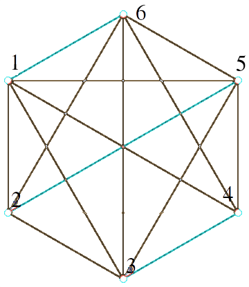
This function is obviously surjective, and far from injective. However, it’s easy to describe the fibers $\inv f(G)$ for a 1-regular graph $G$. Fix any permutation $\sigma$. If we transpose the endpoints of an edge, we don’t change which fiber $\sigma$ belongs to (e.g. $f(341625)=f(346125)$). Similarly, if we permute the edges themselves, then the resulting graph is unaffected (e.g. $f(341625)=f(253416)$). Convince yourself that every permutation giving the same graph under $f$ comes from a series of these moves. Since there are $n/2$ edges whose vertices can be transposed and (the same) $n/2$ edges that can be permutated, we get that each fiber has size $(n/2)!2^{n/2}$. There are $n!$ permutations of $[n]$, so we conclude that the number of 1-regular graphs is

\[\label{count}\begin{align} \frac{n!}{(n/2)!2^{n/2}}. \end{align}\]

If you want, you can view the above argument as an application of burnside’s lemma to the (relevant) action of the group $S_n\by(S_2)^n$ on the set of 1-regular graphs where $S_n$ is the symmetric group of order $n$.

Now that that’s out of the way, we once again want to investigate $\Pr\sqbracks{E(S,\bar S)=\emptyset}$ where $S\subseteq V(G)$. Since the graphs $G_1,\dots,G_m$ are sampled independently, we have

\[\Pr\sqbracks{E(S,\bar S)=\emptyset}=\Pr\sqbracks{E_G(S,\bar S)=\emptyset}=\prod_{i=1}^m\Pr\sqbracks{E_{G_i}(S,\bar S)=\emptyset}\]

Because of the following, we can restrict out attention to such $S$ with even order.

With that said, fix some $i$ and a set $S\subseteq V(G_i)=V(G)$ of even order. Recall that $n=2g$ and write $|S|=2a$ where $a\le g$. Then, to calculate $\Pr\sqbracks{E_{G_i}(S,\bar S)=\emptyset}$, it suffices to simply consider ratio between the number of $1$-regular graphs where this is the case and the total number of $1$-regular graphs ¹¹. Notice that $G_i[S]$ and $G_i[\bar S]$ are both $1$-regular, so we can use equation $(\ref{count})$. Because this is gonna involve a lot of factorials, we’re gonna hop over to a Wikipedia page for Sterling’s approximation, and find something that looks useful.

At this point, I want to remind you that the order of our graph is $n=2g$. This might be easy to forget during what followings. Returning to the problem, the above corollary tells us that

\[\begin{align*} \Pr\sqbracks{E_{G_i}(S,\bar S)=\emptyset} &= \frac{\frac{(2a)!}{a!2^a}\cdot\frac{(2(g-a))!}{(g-a)!2^{g-a}}}{\frac{(2g)!}{g!2^g}} \\ &= \parens{\frac{(2a)!}{a!}}\parens{\frac{(2(g-a))!}{(g-a)!}}\parens{\frac{g!}{(2g)!}} \\ &\le \frac{e^3}2\cdot\frac{(4a)^a(4g-4a)^{g-a}}{(4g)^g} \\ &= \frac{e^3}2\cdot\frac{a^a(g-a)^{g-a}}{g^g} \end{align*}\]

Thus, letting $q_{n,m}=q(G)$ be the probablity that $G$ is disconnected, we have

\[\begin{align} q_{n,m} \le\frac12\sum_{\substack{S\subsetneq V(G)\\S\neq\emptyset}}\Pr\sqbracks{E(S,\bar S)=\emptyset} &=\frac12\sum_{\substack{S\subsetneq V(G)\\S\neq\emptyset}}\prod_{i=1}^m\Pr\sqbracks{E_{G_i}(S,\bar S)=\emptyset} \nonumber \\&=\frac12\sum_{a=1}^{g-1}\binom{2g}{2a}\sqbracks{\frac{e^3}2\cdot\frac{a^a(g-a)^{g-a}}{g^g}}^m \label{bound} \end{align}\]

Like last time, our goal is to show that $q_{n,m}\to0$ as $n\to\infty$ (equivalently, as $g\to\infty$). ¹² Unlike last time, this time we will actually succeed. At this point, it might be a good idea to pause, ¹³ and take some time to try to calculate the limit of this upper bound yourself before taking a look at what I eventually came up with.

This is a pretty nasty expression. Things are not hopeless though; one can check numerically that it does indeed converge to $0$ as $n\to\infty$ (given fixed $m\ge3$). We just need to figure out how to prove this. We will attempt to abstract away the important feasures of this sum and prove convergence to $0$ is a slightly more general setting. First note that the constant factors do not matter, so we just need to show

\[\sum_{a=1}^{g-1}\binom{2g}{2a}\sqbracks{\frac{a^a(g-a)^{g-a}}{g^g}}^m\to0\text{ as }g\to\infty\]

The way I think about this problem, roughly speaking, we have a sum where each summand approaches 0, and we want to show that the whole sum does as well. We would like a theorem along the lines of, “given a function $f(a,g)$ s.t. $\lim_{g\to\infty}f(a,g)=0$ for any fixed $a$, we must have $\lim_{g\to\infty}\sum_{a=1}^gf(a,g)=0$.” However, this is false as stated since one can take ¹⁴ $f(a,g)=a/g$ which satisfies the hypothesis but for which

\[\lim_{g\to\infty}\sum_{a=1}^gf(a,g) = \lim_{g\to\infty}\frac{g+1}2 = \infty.\]

Hence, we’ll need to strengthen our hypotheses if we want to guarantee convergence to $0$. This leads us to the following.

In our particular case of interest, we have

\[\ast h_g(a)=g\binom{2g}{2a}\sqbracks{\frac{a^a(g-a)^{g-a}}{g^g}}^m=\binom{2g}{2a}\cdot\frac{a^{am}(g-a)^{gm-am}}{g^{gm-1}}\]

(when $a < g$). Hence, we just need to prove that this converges uniformly to $0$. In order to do this, we will make use of the following

Now we’re ready to wrap things up. We begin by defining ¹⁵

\[\ast f(a,g):=\twocases{\binom{2g}{2a}\sqbracks{\frac{a^a(g-a)^{g-a}}{g^g}}^m}{a < g}0,\]

and

\[\ast h_g(a):=g\cdot f(a,g)=\twocases{\binom{2g}{2a}\cdot\frac{a^{am}(g-a)^{gm-am}}{g^{gm-1}}}{a < g}0.\]

We claim that $\ast h_g(a)$ uniformly converges to $0$. To see this, note that ¹⁶

\[M_g:=\sup_{a\in\N}\abs{\ast h_g(a)}=\ast h_g(1)=\frac{2g(2g-1)(g-1)^{gm-m}}{2g^{gm-1}}=\frac{(2g-1)(g-1)^{gm-m}}{g^{gm-2}}\le\frac{2(g-1)^{gm-m}}{g^{gm-3}}.\]

At this point, we make a slight concession. Numerical evidence suggests that $(\ref{bound})$ approches $0$ as $n\to\infty$ for any $m\ge3$. However, for $m=3$, we have

\[M_g\le\frac{2(g-1)^{3g-3}}{g^{3g-3}}=2\parens{\frac{g-1}g}^{3g-3}=2\sqbracks{\parens{1-\frac1g}^{g-1}}^3\longrightarrow\frac2{e^3}\text{ as }g\to\infty.\]

Hence, it is possible that $\lim M_g\neq0$ when $m=3$. In brighter news, for $m\ge4$, we have

\[M_g\le\frac{2(g-1)^{gm-4}}{g^{gm-3}}=\frac2g\parens{\frac{g-1}g}^{gm-4}\le\frac2g\parens{\frac{g-1}g}^{4m-4}\longrightarrow0\text{ as }g\to\infty\]

Now (when $m\ge4$), we can climb back up our tower of implications to finally conclude what we want. First, because $\lim M_g=0$, we know that $\ast h_g$ uniformly converges to $0$. This means that

\[\lim_{g\to\infty}\sum_{a=1}^g\frac{\ast h_g(a)}g=\lim_{g\to\infty}\sum_{a=1}^{g-1}\binom{2g}{2a}\sqbracks{\frac{a^a(g-a)^{g-a}}{g^g}}^m=0.\]

Because (a constant multiple of) the above expression (without the limit) gives an upper bound for $q_{n,m}=q_{2g,m}$, we conclude that $\lim_{n\to\infty}q_{n,m}=0$ when $m\ge4$. That is to say that when everyone is pansexual, everyone in a class of students will be married to each other after $\ge4$ of the Marriage Pact almost always ¹⁷.

Going Forward

This still leaves open the question of what happens when we start to allow students to have more restrictive sexual orientations. Resolving the “everyone pansexual” case took longer than I expected, so I will hold off thinking about this harder problem for the time being. Given how things resolved here, I suspect that everyone is likely to end up married to each other given mild assumptions on the distribution of sexual orientations.

To end the post, observe that we can use $(\ref{bound})$ to show that for a class of $1000$ students, after $4$ years, the probablity that everyone is married to each other is at least

\[1-\frac12\sum_{a=1}^{499}\binom{1000}{2a}\sqbracks{\frac{e^3}2\cdot\frac{a^a(500-a)^{500-a}}{500^{500}}}^4\ge99.8\%\]

In other words, the Stanford class of 2021 is gonna be really close.

comments powered by Disqus