Usually in mathematics, you have some question you want answered, and you often want to find a constructive answer. You are questioning if something exists, and so you want an example of it (if it does exist), or you know something exists but want to know how many of them exist, and so you would like a way to easily find multiple examples of it. However, sometimes its easier to come up with a nonconstructive answer where you show something exists (maybe even that many of them do), but you don’t produce even one example of it. Still, nonconstructive answers can provide useful insights ¹.

In this post I want to show a couple examples of what’s called the probabilistic method. The basic idea is you want to study some property of a set of objects. In order to do this, you consider a random distribution over your set of objects, and investigate the probability that a randomly chosen object has the desired property. In particular, the the probability that the object has the property is nonzero, then some object with that property must exist! In this way, you can prove the existence of certain types of objects without needed to construct an example.

Primes

As a warm up, let’s prove something that hopefully doesn’t seem too far-fetched. Before we state, let’s introduce a useful function. Let \(\pi(n)=|\{p\le n:p\text{ is prime}\}|\). That is, \(\pi(n))\) counts the number of primes numbers there are lequal² to \(n\).

Theorem
There are infinitely many prime numbers.

Fix any postive integer \(n\). Consider possible factorizations of all the integers \(k\) with \(1\le k\le n\). Note that each such \(k\) can be factored as \(k=rs^2\)³ where \(r\) is square-free⁴. Since each \(k\) has a unique factorization of this form, if we can get an upper bound for the number of ways of picking \(r\) and \(s\) (such that \(rs^2\le n\)), then we will have an upper bound for the value of \(n\). This is because each such choice corresponds to a different value for \(k\), and so the number of choices is the number of values of \(k\) which is \(n\).

We’ll bound choices for \(s\) and \(r\) separately. Since \(s\) is easier, we’ll start with it. Since \(s^2\le rs^2 = k\le n\), we must have that \(s\le\sqrt n\), and so there are at most \(\sqrt n\) possible choices for \(s\). For bounding \(r\), note that being square-free means that all of its prime factors are unique. Thus, we can count the number of choices for \(r\) by counting the number of choices for its prime factors. Each such choice corresponds to some (finite) set of prime numbers. Since we require that \(r\le rs^2 = k\le n\), every prime in \(r\)’s factorization must be lequal to \(n\). Thus, the possible choices for the primes that make up \(r\) (and hence the possible choices for the values of \(r\)) correspond to subsets of \(\{2, 3, 5, \dots, p\}\) where \(p\) is the largest prime lequal to \(n\). By definition, the size of this set is \(\pi(n)\) and so there are at most \(2^{\pi(n)}\) valid choices for \(r\). Since \(s\) has at most \(\sqrt n\) possible values and \(r\) has at most \(2^{\pi(n)}\) possible values, the factorization \(rs^2\) has at most \(2^{\pi(n)}\sqrt n\) possible choices, and hence \(n\le2^{\pi(n)}\sqrt n\). A little bit of algebra shows that this implies that \(\pi(n)\ge\frac12\log_2(n)\). Since the right hand side approaches infinity as \(n\rightarrow\infty\), there must be infinitely many primes. \(\square\)

I know what you are thinking. I spent the first bit of this post talking about the probabilistic method and how it’s great and junk, but there was no probability in the proof I just presented. This was intentional. See, many probabilstic proofs don’t actually require probability (although it’s often useful to use it), and can be transformed into equivalent proofs purely using counting arguments. Instead of showing the probability of something is positive, you can count how many of them there are, and so that this is positive directly⁵. Now that I have said this, I will present an alternate proof of this theorem that makes explicit use of probability.

We will form a distribution on the numbers \(\{1,2,3,\dots,n\}\) for some fixed positive integer \(n>1\). This distribution will be formed by noticing that all of these numbers can be factored into the form \(rs^2\) where \(r\) is square-free. Our distribution works by picking an \(s\in\{1,2,\dots,\lfloor\sqrt n\rfloor\}\) uniformly. For choosing \(r\), we once again rely on the fact that there exists a 1-1 correspondence between choices of \(r\) and subsets of \(\{2,3,5,\dots,p\}\) where \(p\) is the largest prime lequal to \(n\). As such, \(r\) is chosen by uniformly selecting one of these subsets and taking the product of all its members ⁶. Every choice of \(s,r\) leads to a different number, and every choice of \(s,r\) is equally likely, so our distribution is actually just the uniform distribution on \(\{1,2,3,\dots,n\}\)!⁷ Since we are interested in the number of primes, let’s investigate how likely drawing from this distribution is the give us a prime number. Note that \(rs^2\) is prime iff \(s=1\) and \(r\) corresponds to a singleton set. \(\Pr(s=1)=\frac1{\sqrt n}\) and \(\Pr(r\text{ corresponds to a singleton set})=\frac{\pi(n)}{2^{\pi(n)}}\). Calling these events \(A\) and \(B\), respectively⁸, it is easily seen that \(\Pr(A\mid B)>\Pr(A)\) and so, letting \(X\) be a random variable drawn from this distribution,

\[\begin{align*} \frac{\pi(n)}n = \Pr(X\text{ prime}) = \Pr(A\text{ and }B) = \Pr(B)\Pr(A\mid B) > \Pr(B)\Pr(A) = \frac{\pi(n)}{2^{\pi(n)}\sqrt n} \end{align*}\]

Rearranging this equation shows that \(\pi(n)>\frac12\log_2(n)\), and so we once again have that there are infinitely many primes. \(\square\)

And so we see our counting argument has an equivalent probabilistic argument. I’ll admit that we did not gain many insights from using a probabilistic approach here ⁹, but this was just a warm up and the next proof will rely more on probability.

Graphs

Before getting to the theorem here, I’m gonna do a quick introduction to graph theory.

Definition
A graph is a pair \(G=(V,E)\) where \(V\) is a set of vertices and \(E\subseteq V\times V\) is a set of edges.

Here, we restrict ourselves to simple, undirected graphs. That means that edges go both ways (\((u,v)\in E\iff (v,u)\in E\)), no vertices are adjacent to themselves (for all \(v\in V\), \((v,v)\not\in E\)), and each edge appears at most once (\(E\) is a set and not a multiset).

Definition
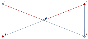
A path in a graph \(G\) from \(u\in V(G)\) to \(v\in V(G)\) is an alternating sequences of vertices and edges \(u=v_0,e_0,v_1,e_1,v_2,\dots,v_{k-1},e_{k-1},v_k=v\) where every edge is unique, and every vertex is unique. The length of a path is its number of edges.

Below is an example of a simple, undirected graph with a path of length 3 highlighted.

Definition
A graph \(G=(V,E)\) is connected if for any distinct \(v,u\in V\), there exists a path in \(G\) from \(v\) to \(u\).

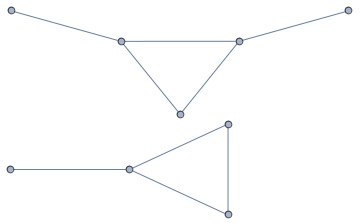
The graph above is connected. The graph below is not connected.

Definition
A graph \(G=(V,E)\) is \(k\)-edge-connected for a positive integer \(k\) if you must remove \(k\) edges in order to disconnect it. More formally, for any \(F\subseteq E\) with \(|F|<k\), the graph \((V,E-F)\) is connected. In particular, a graph is 1-edge-connected if and only if it is connected.

Now that we have all these definitions, we are almost ready to state the theorem. First, we say almost all graphs satisfy a given property if the probability that a random graph on \(n\) vertices satisfies this property approaches 1 as \(n\) approaches infinity. In other words, if as you consider more and more graphs, you start to become guaranteed than one chosen at random satisfies the property, then almost all graphs satisfy that property. We now just need to formalize what we mean by random graph.

Definition
Fix some number \(0<p\le1\). The Erdős–Rényi random graph on \(n\) vertices is constructed by choosing each of the \(\binom n2\) possible edges independently where each edge appears with probability \(p\).

Note that although we usually talk about a random graph, or the random graph, we actually definied a distribution on graphs, and what we mean by a random graph is some graph drawn from this distribution. Also note that for \(p=\frac12\), we get the uniform distribution on simple, undirected graphs with \(n\) vertices. Finally, the theorem.

Theorem
For any positive integer \(k\), and any choice of \(p\) with \(0<p\le 1\), almost all graphs are \(k\)-edge-connected.

Fix a choice of \(k\) and \(p\), and consider an Erdős–Rényi random graph \(G\) with \(n\) vertices and any \(S\subseteq V(G)\). Denote by \(E(S,\bar S)\) the set of edges where exactly one of its vertices is in \(S\). Note that \(G\) is not \(k\)-edge-connected iff \(\mid E(S, \bar S)\mid < k\) for some \(S\). Thus, we will investigate \(\Pr(\mid E(S, \bar S)\mid < k)\). Let \(m=\mid S\mid\), so there are at most \(m(n-m)\) edges in \(E(S, \bar S)\). Using the union bound, we have that

\[\begin{align*} \Pr(\mid E(S, \bar S)\mid < k) &\le \sum_{c=0}^{k-1}\Pr(\mid E(S, \bar S)\mid = c)\\ &= \sum_{c=0}^{k-1}\binom{m(n-m)}cp^c(1-p)^{m(n-m)-c}\\ &= (1-p)^{m(n-m)}\sum_{c=0}^{k-1}\binom{m(n-m)}c\left(\frac p{1-p}\right)^c \end{align*}\]

Now that we have this, let \(q_n\) be the probability that \(G\) is not \(k\)-edge-connected. Summing over all possible \(S\subseteq V(G)\), we have¹⁰

\[\begin{align*} q_n\le\frac12\sum_{m=1}^{n-1}\left[\binom nm(1-p)^{m(n-m)}\sum_{c=0}^{k-1}\binom{m(n-m)}c\left(\frac p{1-p}\right)^c\right] \end{align*}\]

We want to show that almost all graphs are \(k\)-edge-connected, so we want to show that \(\lim_{n\rightarrow\infty}q_n=0\). As things are right now, \(q_n\) does not look particularly nice to work with, so prepare for some bounds. First note that since this expression is symmetric in \(m\) and \((n-m)\), we can sum up to \(\lfloor n/2\rfloor\) and multiply by 2 to get the same result. Furthermore, for \(m\le n/2\) we have that \((1-p)^{n-m}\le(1-p)^{n/2}\) and that \(\binom nm\le n^m\) ¹¹. Using these facts, we get

\[\begin{align*} q_n\le \sum_{m=1}^{\lfloor n/2 \rfloor}\left[n^m((1-p)^{n/2})^m\sum_{c=0}^{k-1}\binom{m(n-m)}c\left(\frac p{1-p}\right)^c\right]= \sum_{m=1}^{\lfloor n/2 \rfloor}\left[(n(1-p)^{n/2})^m\sum_{c=0}^{k-1}\binom{m(n-m)}c\left(\frac p{1-p}\right)^c\right] \end{align*}\]

Focussing on the sum over \(c\), note that \(\binom{m(n-m)}c\le\binom{n^2}c\le(n^2)^c\) when \(m\le n/2\). Thus

\[\begin{align*} \sum_{c=0}^{k-1}\binom{m(n-m)}c\left(\frac p{1-p}\right)^c\le \sum_{c=0}^{k-1}(n^2)^c\left(\frac p{1-p}\right)^c= \sum_{c=0}^{k-1}\left(\frac{pn^2}{1-p}\right)^c \end{align*}\]

Still focussing on this sum, note that its largest term is roughly \(n^{2k-2}\). Thus, for sufficiently large \(n\), this sum is less than \(n^{2k}\) and since \(m\ge1\), the sum is also less than \(n^{2km}\). Thus, for such large \(n\),

\[\begin{align*} q_n\le \sum_{m=1}^{\lfloor n/2 \rfloor}\left[(n(1-p)^{n/2})^mn^{2km}\right]= \sum_{m=1}^{\lfloor n/2 \rfloor}\left[(n^{2k+1}(1-p)^{n/2})^m\right] \end{align*}\]

Finally, note that \(0\le1-p<1\) and so, for sufficiently large \(n\), \(n^{2k+1}(1-p)^{n/2}<1\). For such \(n\), we have

\[\begin{align*} q_n\le \sum_{m=1}^\infty\left[(n(1-p)^{n/2})^mn^{2km}\right]= \frac{n^{2k+1}(1-p)^{n/2}}{1-n^{2k+1}(1-p)^{n/2}} \end{align*}\]

As \(n\rightarrow\infty\), the right hand side of this inequality approaches 0. Since the right hand side is an upper bound, and \(q_n\ge0\) for all \(n\), this shows that \(\lim_\limits{n\rightarrow\infty}q_n=0\) as desired. Hence, almost all graphs are \(k\)-edge-connected. \(\square\)

comments powered by Disqus