One of the first “theorems” I heard about was The Fundamental Theorem of Algebra, and I remember being kind of drawn to it for a long time after first seeing it. I think this was less because of the statement of the theorem itself, and more because the word fundamental in its title made it seem really important and imposing ¹. Either way, I was convinced for a long time that it was somehow a mysterious theorem, that although easy to state, must have one of those impossible to understand, complicated proofs; the kind of thing that’s proved once via a lot of effort, and then is just applied afterwards without many people wanting to return to the proof because it’s just that out there. Despite this, my fascination with it made me determined to see and understand its proof once I became really good at/knowledgable of math. Luckily for me, I was wrong. The proof of the theorem is not arcane. In fact, there are many proofs of it, some of which even I can understand.

Before getting into a proof, let’s quickly state the theorem and then move on

The Fundamental Theorem of Algebra
If $p(x)=a_nx^n+a_{n-1}x^{n-1}+\dots+a_1x+a_0$ is any polynomial with complex coefficients, then $p(x)$ has a zero in $\mathbb C$.

Intro to $\mathbb C$

If the idea of number $i$ such that $i^2=-1$ doesn’t frighten or anger you, then skip this section. If not, I’m going to somewhat quickly try to convince you that this is ok.

One way to think of complex numbers is to view them as a way of doing geometry via arithmetic. Let’s say, for example, you are making a 2D game, and in this game you probably want to keep track of positions of different objects, so you represent positions as points in the plane. Each object has some position $(x,y)\in\mathbb R^2$. You probably want objects to move, so along with a position, every object needs some velocity $(dx,dy)\in\mathbb R^2$. Now, you can move objects by adding their velocity to their position, so after one timestep their position becomes $(x+dx,y+dy)$. Simple enough. Objects in your game also rotate around each other². Originally, you might handle this by having some angle $\theta$ of rotation for an object, and then updating its poition via some complicated formula involving $\sin$ and $\cos$. This is kinda messy, but then you remember how well representing things as points worked for moving things around before, and so you store rotations as a point $(\cos\theta,\sin\theta)$ on the unit circle. You then need some operation $\cdot$ such that $(x,y)\cdot(\cos\theta,\sin\theta)$ gives the rotation of $(x,y)$ (about the origin. To rotate about a different point, you just translate, rotate, then translate back). Once you do this, you’ll likely want to extend $\cdot$ such that $(x,y)\cdot(a,b)$ makes sense for all points in the plane, and not just onces where $(a,b)$ is on the unit circle. Motivated by the fact that $5*(x,y)$ scales $(x,y)$ by a factor of 5, and $0.5*(x,y)$ scales it by a factor of $1/2$, you say that $(x,y)\cdot(a,b)$ rotates $(x,y)$ by the angle $(a,b)$ makes with the $x$-axis, and then scales us by the distance of $(a,b)$ from the origin.

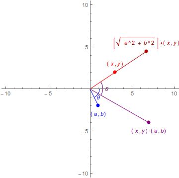
This turns out to be pretty useful because it lets you combine two transformations into one, and this $\cdot$ operation plays really nicely with adding points. In fact, if you do the math to work things out, you will see that $(x,y)\cdot(a,b)=(xa-yb,xb+ay)$ which means that $(x,0)\cdot(y,0)=(xy,0)$ so the $x$-axis is really just the real number line, and $(0,1)\cdot(0,1)=(-1,0)$ so you have a number whose square is $-1$! By trying to create an arithmetic that allows us to do geometric transformations, we naturally find ourselves actually manipulating complex numbers where $a+bi\leftrightarrow(a,b)$. I probably should mention that complex number actually usually aren’t used for rotations and such in 2D games, but an extension of them called quaternions are used for rotations in 3D games.

If that’s not convincing, then another perspective on complex numbers is that you are really just doing clock arithmetic when you work with them. When doing math with time, you wrap around every 12 (or 24) hours, so you are really just treating 12 as if it were 0, and then doing normal math (Ex. $4+10=14=12+2=2$ so $10$ hours past $4$ is $2$). With complex numbers, you are doing something similar. You are doing normal math with polynomials (with real coefficients), except you treat the polynomial $x^2+1$ as being zero. So, for example, when you say $(3+4i)(5-2i)=23+14i$, this is really because

\[\begin{align*} (3+4x)(5-2x) = 15 + 14x - 8x^2 = 15 + 14x - 8(x^2+1) + 8 = 23 + 14x \end{align*}\]

Symbolically, in case you’ve studied some abstract algebra but not seen this,

\[\begin{align*} \mathbb C\simeq\frac{\mathbb R[x]}{(x^2+1)} \end{align*}\]

Definitions and Junk

Now that we have that out of the way, before moving on to the proof itself, we need to setup some notation, definitions, and lemmas, so let’s get to that. In the below definitions, $X$ is an arbitrary subset of $\mathbb C$.

Definition
A path is a continuous function $f:[0,1]\rightarrow X$. Furthermore, if we have that $f(0)=f(1)$, then we call $f$ a loop based at $f(0)$.

An important thing to know about paths is that you can compose them. If you have two paths $f,g:[0,1]\rightarrow X$ where $f(1)=g(0)$, then you can form a new path $g\cdot f:[0,1]\rightarrow X$ where you first do $f$, then do $g$. In order to keep the domain $[0,1]$, you have to traverse $f$ and $g$ at twice the normal speed, but that’s really just a technicality³.

Note that for some reason I think in terms of paths more easily than I do in terms of loops, so although we’ll be dealing exclusively with loops here, I will often forget and say path instead.

Notation
Let $S^1=\{z\in\mathbb C:|z|=1\}$ be the unit circle in the complex plane

Quick remark: Notice that there is a 1-1 correspondence between loops and continuous circle functions $f:S^1\rightarrow X$ since a circle is really just a line segment with its endpoints glued together. I may end up switching between these two perspectives during this post.

The proof of the fundamental theorem we’ll present is pretty dependent on loops. The basic idea is that if you have a polynomial without a zero, then you can find a “constant loop that circles the origin multiple times”. I use quotes because this is not exactly what we’ll show, but basically it. In either case, if a loop is constant it doesn’t move so there’s no way it could circle the origin even once, and so contradiction. We need a mathematically precise way of defining what it means to “circle the origin multiple times”, and for that, we’ll use a little homotopy theory.

Definition
Given two paths $f:[0,1]\rightarrow X$ and $g:[0,1]\rightarrow X$ with the same basepoints (i.e. $f(0)=g(0)$ and $f(1)=g(1)$), a homotopy $H:[0,1]\times[0,1]\rightarrow X$ from $f$ to $g$ is a continuous⁴ function such that $H(t,0)=f(t)$ and $H(t,1)=g(t)$ for all $t\in[0,1]$, and $H(0,s)=f(0)$ and $H(1,s)=f(1)$ for all $s\in[0,1]$. If there exists a homotopy $H$ from $f$ to $g$, then we say $f$ and $g$ are homotopy equivalent, and denote this $f\sim g$.

You can think of a homotopy as a continuous deformation from one path into the other. Something like this

Remark
One important example of a homotopy is the one depicted above. This is the so-called staright line homotopy, and is the result of thinking of your paths as points and then drawing a line between them. For $f,g:[0,1]\rightarrow X$ paths between the same points, you can define $H(t,s)=(1-s)f(t) + sg(t)$. This is almost always continuous.

Question
When does the straight line homotopy fail to be a homotopy?

Exercise
Show that homotopy equivalence is an equivalence relation.

In this upcoming section, we’ll apply homotopy to loops to see that every loop around a circle has a well-defined number of times it goes around. This will then lead us to the proof of the theorem.

Circles and Degrees

Here, we will study loops $f:[0,1]\rightarrow S^1$ around the unit circle. In general, these things can behave annoyingly by stopping in place, backtracking, etc. so to get a handle on them, we’ll homotope all our paths into nice loops. To that end, let $\omega_n:[0,1]\rightarrow S^1$ be the path $\omega_n(t)=e^{2t\pi in}$ that goes around the unit circle $n$ times where we made use of Euler’s formula.

Our goal is to show that any loop $f:[0,1]\rightarrow S^1$ is homotopic to exactly one “nice” loop $\omega_n$. We will then let the degree of $f$ be $\deg f=n$, and this will be our characterization of the number of times $f$ travels around the unit circle ⁵. In order to do this, we’ll make use of a special function⁶

\[\begin{matrix} p: &\mathbb R &\longrightarrow &S^1\\ &r &\longmapsto &\cos(2\pi r)+i\sin(2\pi r) \end{matrix}\]

What makes this function special is that is allows us to “lift” loops in $S^1$ up to paths in $\mathbb R$. This function is far from injective, but it maps every unit interval in $\mathbb R$ around the circle in a “nice” way. If we look at any (connected) neighborhood around a point on our circle, there are many disjoint copies of that neighborhood in $\mathbb R$ that get mapped into it by $p$. This means that $p$ in some sense has multiple local inverses of any neighborhood in $S^1$. These local inverses are what allow us to lift loops up to $\mathbb R$. Specifically,⁷

Lemma
For any path $f:[0,1]\rightarrow S^1$, there exists a unique lift $\tilde f:[0,1]\rightarrow\mathbb R$ such that $p\circ\tilde f=f$ and $\tilde f(0)=0$.

Pf: Let $f:[0,1]\rightarrow S^1$ be a path. The remark I made above on local inverses can be said more formally as this: for any point $x\in S^1$, there exists a neighborhood $N$ of $x$, called an elementary neighborhood, such that each path component of $p^{-1}(N)$ is mapped homeomorphically onto $N$. Let $\{U_i\}_{i\in I}$ be a collection of elementary neighborhoods that cover $S^1$, so $\{f^{-1}(U_i)\}_{i\in I}$ is an open cover of the compact metric space $[0,1]$, which means it has some finite subcover $\{V_j\}_{j=1}^n\subseteq\{f^{-1}(U_i)_{i\in I}\}$. Furthermore, it is a fact that I will not prove here that you can find a natural $m\in\mathbb N$ such that each of the images $f([0,1/m]),f([1/m,2/m]),\dots,f([(m-1)/m,1])$ is completely contained in some elementary neighborhood $W_j$. To simplify notation, let $x_j=j/m$ and $I_j=[x_j,x_{j+1}]$. Now, we can lift $f$ by lifting it piece by piece. For each $j\in\{0,1\dots,m-1\}$, we can form a unique path $g_j:I_j\rightarrow\mathbb R$ such that $p\circ g_j=f\mid_{I_j}$ since $f(I_j)$ is contained in an elementary neighborhood $W_j$ which has exactly one "local inverse" $V_j$ containing $g_{j-1}(x_j)$ and so contains a unique path beginning at $g_{j-1}(x_j)$ that lifts $f\mid_{I_j}$ contained in $U_j$. Thus, our unique lift of $f$ is $\tilde f=g_{m-1}g_{m-2}\dots g_2g_1g_0$. $\square$

That may not have been put perfectly clearly because it’s a proof that is best digested with accompanying visuals, but I am not going through the trouble of making some. One thing I did not make explicit is that we take $g_{-1}(x_0)=0$ in order to comply with $\tilde f(0)=0$. Another thing to keep in mind is that we form our lift by breaking the path up into small pieces, lifting those, then joining them together. If we get a piece $I_j$ of our path small enough to be contained in an elementary neighborhood, then the fact that it has one local inverse containing the point our path left off at means there is a unique way to extend the path. This follows from the fact that each local inverse (i.e. path component) is mapped homeomorphically onto $W_j$, so there’s a unique lift for everything.

For the purpose of the secion, let $1+0i$ be a distingueshed point in the sense that all loops around the circle begin and end there.

Lemma
Let $f:[0,1]\rightarrow S^1$ be a loop based at $1$, and let $\tilde f$ be its unique lift. Then, $\tilde f(1)$ is an integer. We call this integer the degree of $f$.

Pf: $p(\tilde f(1))=f(1)=1$ so $\tilde f(1)\in p^{-1}(1)=\mathbb Z$. $\square$

If you notice, I just redefined degree, so we better hope these definitions are equivalent. Clearly, $\deg\omega_n=n$ since $\tilde\omega_n$ is just a straight path from $0$ to $n$, so we will show these definitions are equivalent via the following lemmas

Lemma
The degree of a path is homotopy-invariant. That is, if $f\sim g$, then $\deg f=\deg g$.

Before we get to the proof, let’s look at a picture of what’s going on here.

We have a path $f$ going around the circle (here $f=\omega_2$), and by using local inverses of $p$, we lift this to a path in $\mathbb R$ from $0$ to $2$. This captures the fact that this circle loop makes two full revolutions around the circle. The idea behind the proof is similar to the proof of paths having unique lefts. You essentially show that you can also lift homotopies, so if $f\sim g$, then $\tilde f\sim\tilde g$ which means they have the same endpoints.

Pf: Exercise for the reader.

Lemma
The converse holds: If $\deg f=\deg g$, then $f\sim g$.

Pf: Let $f,g:[0,1]\rightarrow S^1$ be loops such that $\deg f=\deg g$. Let $\tilde f,\tilde g:[0,1]\rightarrow\mathbb R$ be their respective lifts and note that $\tilde f(1)=\tilde g(1)$. Let $\tilde H:[0,1]\times[0,1]\rightarrow\mathbb R$ be the straight line homotopy $\tilde H(t,s)=(1-s)\tilde f(t)+s\tilde g(t)$, and define $H:[0,1]\times[0,1]\rightarrow S^1$ by $H(t,s)=p\circ\tilde H(t,s)$. Then, $H$ is continuous since it is a composition of continuous functions. Furthermore, $H(t,0)=p\circ\tilde f(t)=f(t)$, $H(t,1)=p\circ\tilde g(t)=g(t)$, $H(0,s)=p(0)=1=f(0)=g(0)$ and $H(1,s)=p(\tilde f(1))=1=f(1)=g(1)$ for all $t,s\in[0,1]$. Thus, $H$ is a homotopy so $f\sim g$. $\square$

Remark
We’ve just shown that any loop around the circle is completely characterized (up to homotopy which is really all that matters) by a single integer, the number of times it goes around. Furthermore, it is easily shown that this integer is additive in the sense that $\deg(fg)=\deg f+\deg g$ (It’s enough to show this for the case that $f=\omega_n$ and $g=\omega_m$ which is obvious), so the structure of loops around the circle is the additive structure of the integers! This is pretty amazing, and can be used to prove some interesting stuff⁸

Proof at Last

At this point, we’ve developed everything we need. Before we get to the proof, let’s “strengthen” our assumptions a little bit. Let $f_0(x)=a_nx^n+a_{n-1}x^{n-1}+\dots+a_1x+a_0$ be any polynomial. Note that we can divide through by $a_n$ without changing the zeros of this polynomial, so we only need to investigate monic polynomials like $f_1(x)=x^n+b_{n-1}x^{n-1}+\dots+b_1x+b_0$ where $b_i=a_i/a_n$. Furthermore, we can replace $x$ with any invertible transformation, and although we change the zeros, we’re still able to recover all the ones we started with. Hence, we can pick $N\in\mathbb R$ small enough that $\mid Nb_{n-1}\mid+\dots+\mid N^{n-1}b_1\mid+\mid N^nb_0\mid<1$ and then consider polynomials like $f_2(x)=N^nf_1(x/N)=x^n+c_{n-1}x^{n-1}+\dots+c_1x+c_0$ where $c_i=N^{n-i}b_i$. This limits the type of polynomials enough that we can state the theorem as

Fundamental Theorem of Algebra
Let $f(x)=x^n+a_{n-1}x^{n-1}+\dots+a_1x+a_0$ be any polynomial with complex coefficients (whose degree $n>0$) such that $\mid a_{n-1}\mid+\dots+\mid a_1\mid+\mid a_0\mid<1$. Then, there exists some $x_0\in\mathbb C$ with $f(x_0)=0$.

Pf: Suppose that $f(x)$ has no zero in $\mathbb C$, so we can regard $f$ as a function from $\mathbb C$ to $\mathbb C-\{0\}$. Now, define a function $g:S^1\rightarrow S^1$ by $g(x)=\frac{f(x)}{\mid f(x)\mid}$, and note that we can equivalently view $g$ as a loop in $S^1$, so $g$ has a well-defined degree. Let $D=\{z\in\mathbb C:|z|\le1\}$ be the unit disc, and note that, representing complex numbers in polar form, we can similarly define $$\begin{matrix} G: &D &\longrightarrow &S^1\\ &re^{2\pi i\theta} &\longmapsto &\frac{f(re^{2\pi i\theta})}{\mid f(re^{2\pi i\theta})\mid} & 0\le r \le 1 &0\le\theta\le 1 \end{matrix}$$ so we can think of $G$ as a function from $[0,1]\times[0,1]\rightarrow S^1$ (the first argument is $r$ and the second $\theta$). Thus, defining $H:[0,1]\times[0,1]\rightarrow S^1$ by $H(t,s)=G(s,t)$ makes $H$ a homotopy! Clearly, $H(t,1)=G(1,t)=g(t)$ (where we view $g$ as a loop instead of as a circle function) and $H(t,0)=G(0,t)=f(0)/\mid f(0)\mid$ for all $t\in[0,1]$, so $g$ is homotopic to a constant function and $\deg g=0$. However, we can also define the following $$\begin{matrix} H': &[0,1]\times[0,1] &\longrightarrow &S^1\\ &(t,s) &\longmapsto &\frac{z^n + s(a_{n-1}z^{n-1}+\dots+a_1z+a_0)}{\mid z^n + s(a_{n-1}z^{n-1}+\dots+a_1z+a_0)\mid} & z=e^{2\pi it} \end{matrix}$$ This function is continuous since its the composition of a bunch of continuous functions, and it is well-defined since the denominator is never 0 $$\begin{align*} \mid z^n + s(a_{n-1}z^{n-1}+\dots+a_1z+a_0)\mid &\ge |z|^n - s|a_{n-1}z^{n-1}+\dots+a_1z+a_0|\\ &\ge |z|^n - s(|a_{n-1}||z^{n-1}|+\dots+|a_1||z|+|a_0|)\\ &= 1 - s(|a_{n-1}|+\dots+|a_1|+|a_0|)\\ &> 1 - s\\ &\ge 0 \end{align*}$$ Now, we just need to note that $H'$ is a homotopy from $[t\mapsto z^n]=[t\mapsto e^{2\pi itn}]=\omega_n$ to $g$, so $\deg g=n$, but this is a contradiction, and hence our initial assumption about $f$ having a zero must be wrong. $\square$

Corollary
Let $f(x)$ be a degree $n$ polynomial with coefficients in $\mathbb C$. Then, $f$ has exactly $n$ (not necessarily distinct) zeros.

Pf: By the theorem, $f$ has some zero $z_0\in\mathbb C$, so let's divide $f$ by $z-z_0$. Using long division, we get some polynomials $q(z),r(z)$ such that $f(z)=q(z)(z-z_0)+r(z)$ and $\deg r(z)<\deg(z-z_0)=1$ or $r(z)=0$ which means $r(z)$ is a constant. Since $0=f(z_0)=q(z_0)(z_0-z_0)+r(z_0)=r(z_0)$, we must have $r(z)=0$ so $f(z)=q(z)(z-z_0)$ and $\deg q(z)=n-1$. Now just apply induction to get that $q(z)$ has $n-1$ zeros, so $f(z)$ has $n$ zeros. $\square$

Finally, an exercise.

Exercise
Where does the argument for the main theorem fail if $f$ has a zero? Since, $f$ has exactly $\deg f$ zeros, you can always find a closed disc on which $f$ has no zero, so why don’t we always get a contradiction?

I’ve seen many other fundamental theorems besides this one, and I am very confused by how a theorem gets to be called fundamental ↩
Maybe it’s a space game, or maybe you have enemies that circles a base to protect it, or maybe etc. ↩
Once we introduce homotopy, we’ll have an equivalence relation on paths. This has the effect that the set of (equivalence classes of) loops based at a single point forms a group called the fundamental group of X. Secretly, this post is really just exploring the fundamental group of the circle. Without homotopy, composition of paths isn’t associative because of the whole doubling speed thing. ↩
Throughtout this post, I will avoid the issue of defining what a continuous function is, because doing so properly requires defining a topology on a set and that’s just too out of the way for this post. You can think of continuity intuitively as meaning nearby inputs get mapped to nearby outputs ↩
Since w_n*w_m=w_{n+m}, this will also show that the fundamental group of the circle is Z, the set of integers ↩
Secretly, this is a covering function, and R is the universal covering space of S^1 ↩
This proof may actually require some, but not much, background in topology. ↩
the fundamental theorem of algebra of course, but also, for example, Brouwer’s Fixed Point Theorem. Brouwer’s theorem then can be used to show the existence of Nash Equilibria in normal form games (think first form of Prisoner’s Dilema shown in my post on it), and from there you get like all of game theory. ↩

Thoughts of a Programmer

Code, Math, Maybe some other stuff

Fundamental Theorem of Algebra

Intro to \(\mathbb C\)

Definitions and Junk

Circles and Degrees

Proof at Last